8-15 944 views
作者:nenn(百度id:正正正正正好)
注1:本文中提到的所有Minecraft版本均为1.12。
注2:相关数学推导需要高等数学知识(大学理工科专业一年级内容),涉及求导、微分和积分的计算。
1.饱和动量下水平阻尼直轨(II类铁轨)上矿车运动的数学模型
通过数学建模,可以摸清任何种类的矿车在I类铁轨上运动的每一个细节[1]。这一数学的模型的意义就在于可以极大提高II类铁轨的研究效率。
我们不妨假设对于II类铁轨可以使用完全类似的数学模型,如此一来,只需要进行一次测量,获得p-F 和p-t 关系图线,就可以获知其他物理量的所有细节。所以不妨设计实验,首先让矿车都达到饱和动量,然后逐渐在II类铁轨上减速。通过entitydata检测[2]获得实验数据。幸运的是,II类铁轨的p-F 关系图线仍然存在明显的线性关系,这意味着I类矿车和II类矿车具有相似的运动规律。
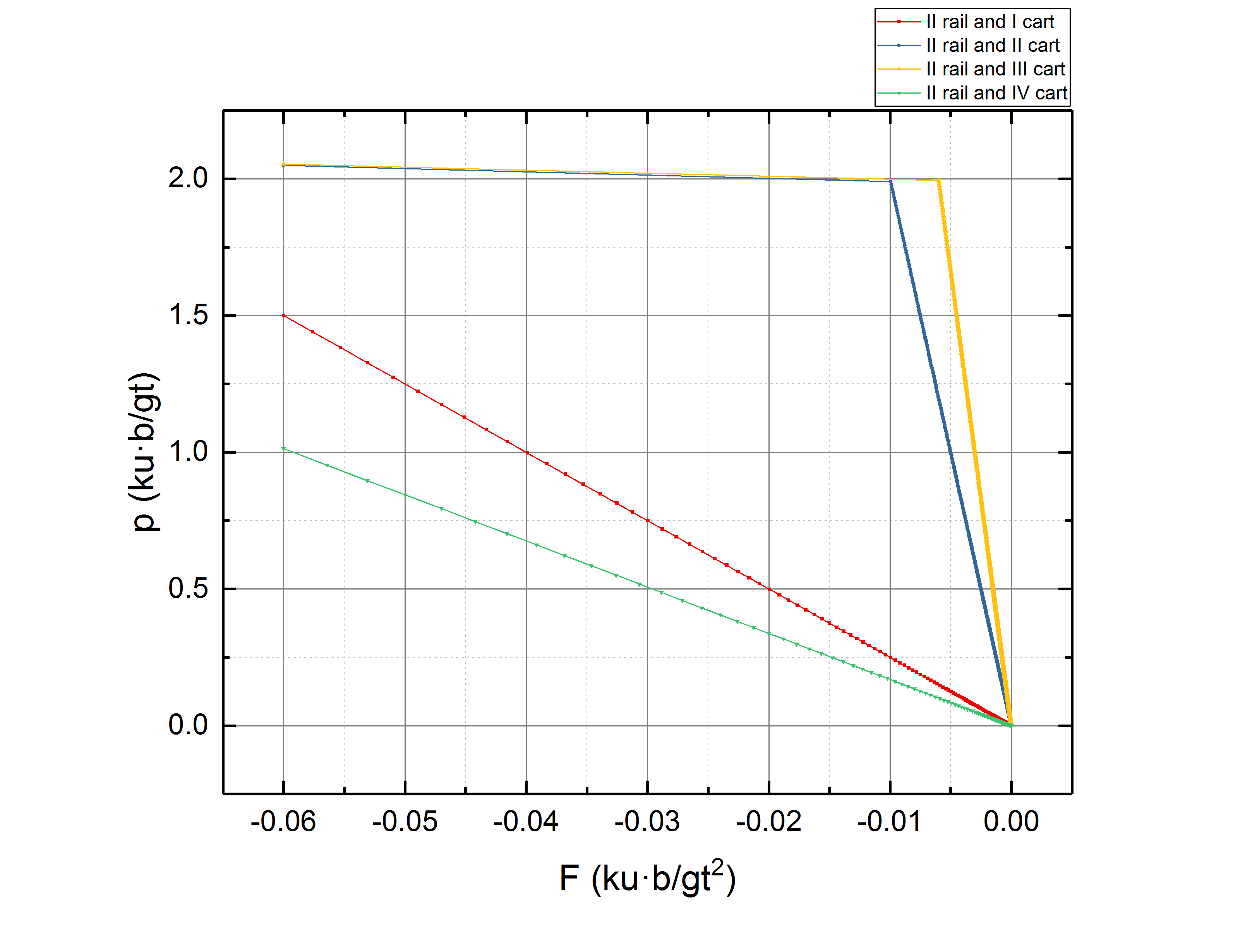
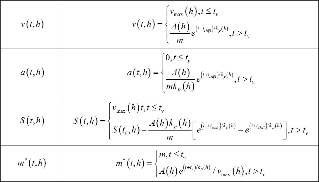
通过整理,可以获得水平阻尼直轨(II类铁轨)上矿车运动的数学模型:
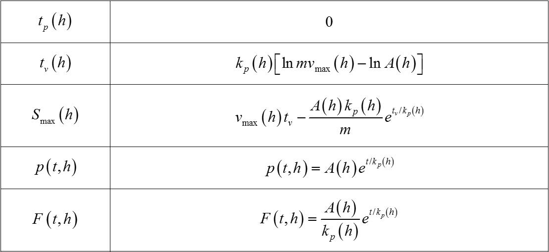
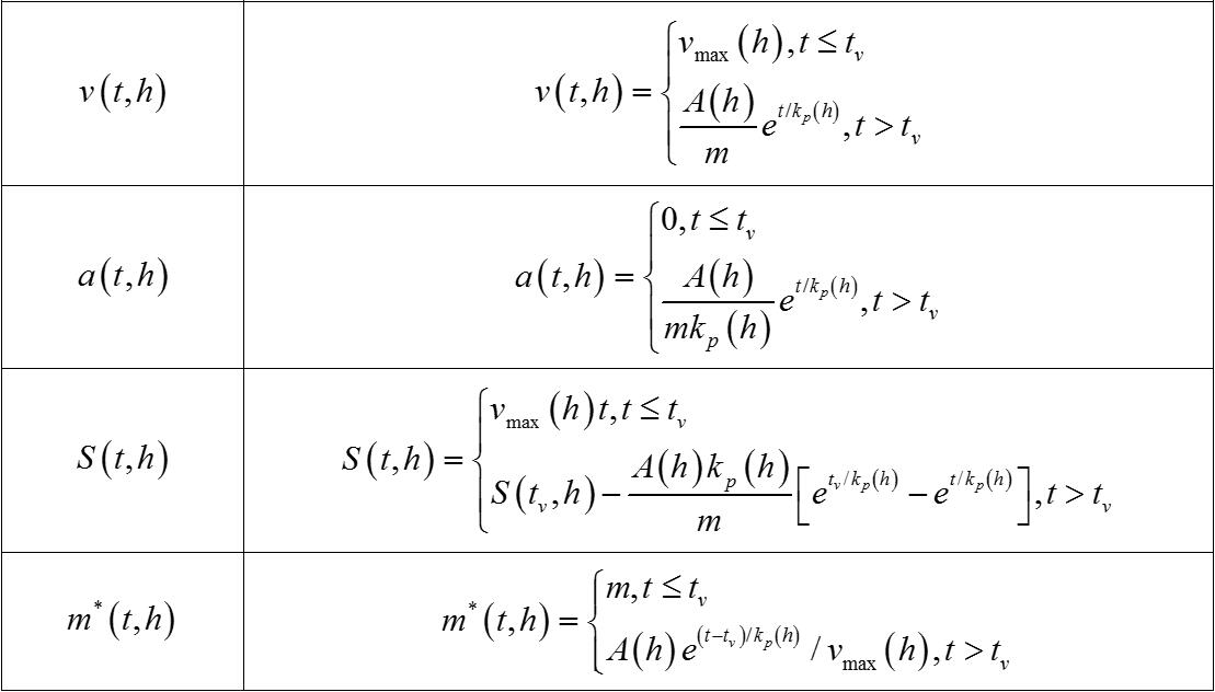
模型中的参数如下:
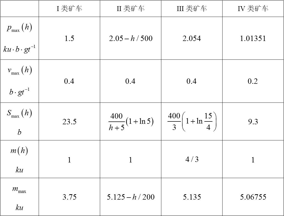
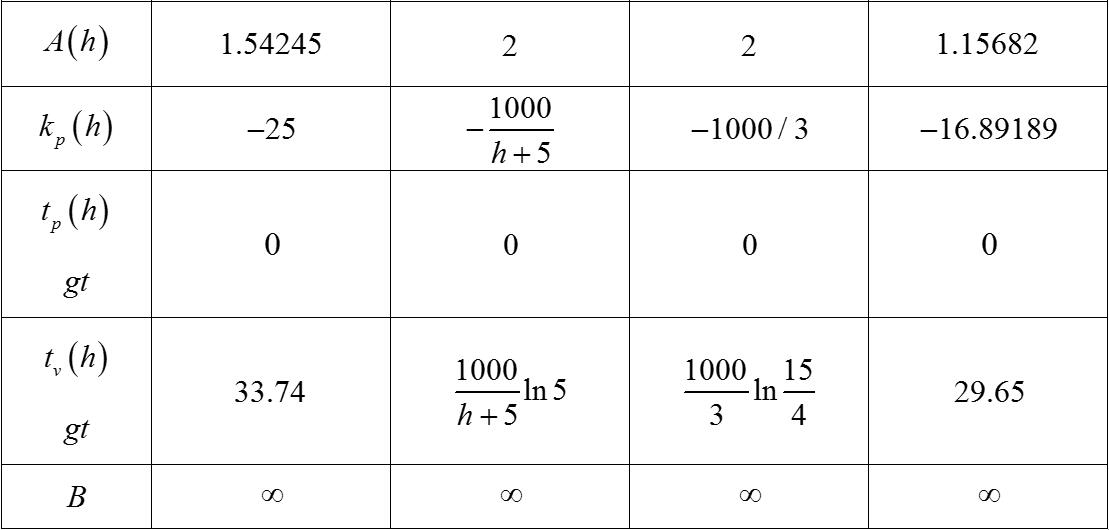
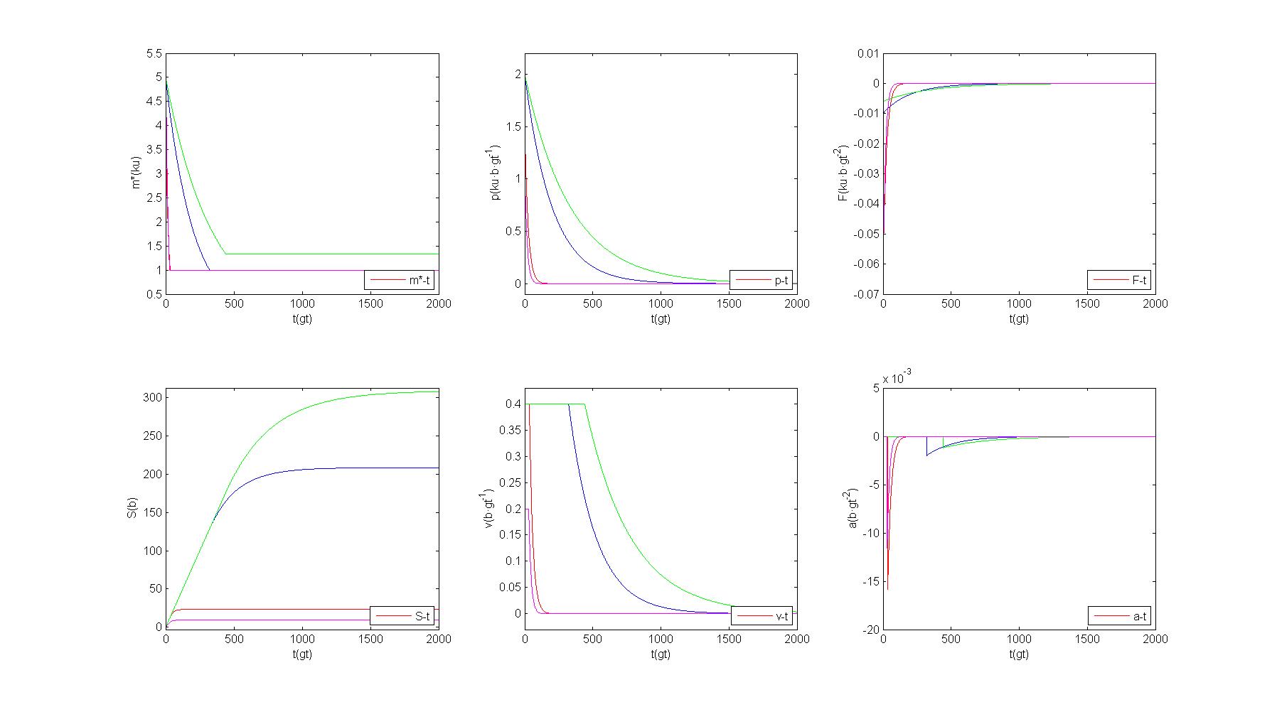
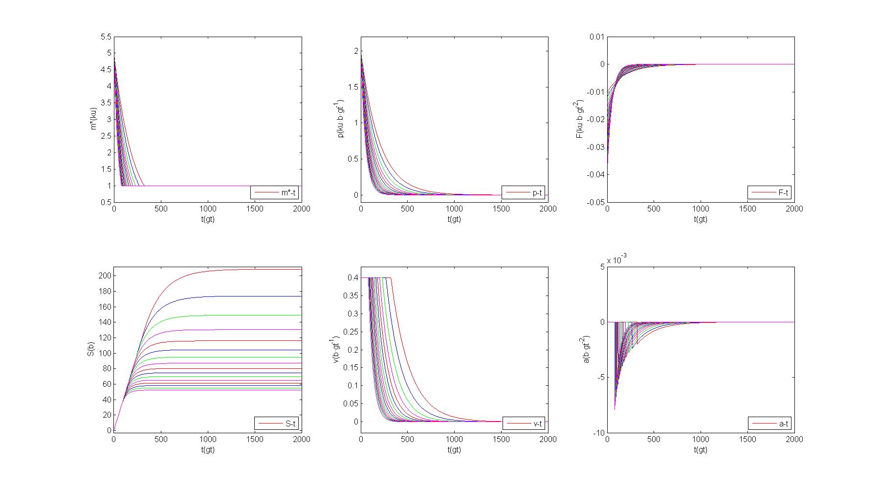
同样可以通过Matlab验证模型的正确性:
实验中还可以观察到一个有趣的现象,也就是矿车只有到达了铁轨中心后,矿车才会认为到达了这段铁轨上,这段铁轨才会对矿车产生作用。在矿车未达到这一段铁轨中心时,矿车依然会认为自己处在这段铁轨相邻的轨道上。
3.非饱和动量情况下数学模型的扩展
我们不妨假设,上述从饱和动量情况下获得的数学模型同样适用于非饱和动量的情况,这是因为矿车并没有一个明确的标记标注其本身是否到达了饱和动量的状态。如此只要对之前的数学模型略加修改,就可以获得水平阻尼直轨(II类铁轨)上矿车的运动学和动力学规律。
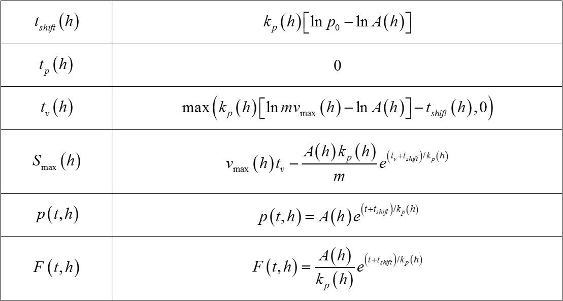
由于所有的物理量都可以通过p-t 关系获得,而p-t 关系满足p(t,h)=A(h)exp[t/tp(h)] ,因此如果进入阻尼直轨时的动量p 小于饱和动量pmax 时,可以理解为矿车已经经过了一段虚构的阻尼直轨作用后到达了这一状态。我们假设矿车从饱和动量状态到达目前状态经过了时间tshift ,那么,就可以通过进入阻尼直轨时的动量p 获得tshift 的值。
如此,只要将(t+tshift) 的值替换上面模型中的t ,即可获得扩充后的数学模型。这样一来,只需要知道进入阻尼直轨时的动量p ,就可以知道矿车在阻尼轨道上所有物理量的动态过程。
4.Matlab代码
1)定义IIrails函数
function [OU] = IIrails(Kind,h,t,p0,na)

%设置初始参数

pmax=[1.5, 2.05-h./500, 2.054, 1.01351];

vmax=[0.4, 0.4, 0.4, 0.2];

m=[1, 1, 4/3, 1];

A=[1.54245, 2, 2, 1.15682];

kp=[-25, -1000./(h+5), -1000./3, -16.89189];

%计算其他参数

tshift=kp(Kind).*log(p0./A(Kind));

tv=max(kp(Kind).*log(m(Kind).*vmax(Kind)./A(Kind))-tshift,0);

Smax=vmax(Kind).*tv-A(Kind).*kp(Kind)./m(Kind).*exp(tv./kp(Kind));

mmax=p0./max(vmax(Kind),p0./m(Kind));

%计算p,F,S,v,a

p=A(Kind).*exp((t+tshift)./kp(Kind));

F=A(Kind)./kp(Kind).*exp((t+tshift)./kp(Kind));

Ss=tv.*vmax(Kind);

S=(1-sign(t-tv))./2.*vmax(Kind).*t+(1+sign(t-tv))./2.*(Ss-A(Kind).*kp(Kind)./m(Kind).*(exp((tv+tshift)./kp(Kind))-exp((t+tshift)./kp(Kind))));

v= min(A(Kind)./m(Kind).*exp((t+tshift)./kp(Kind)),vmax(Kind));

a=(1+sign(t-tv))./2.*A(Kind) ./m(Kind)./kp(Kind).* exp((t+tshift)./kp(Kind));

%函数输出

temp=[p,F,S,v,a,tv,Smax,pmax(Kind),vmax(Kind),m(Kind),mmax,A(Kind),kp(Kind)];

switch na

case 'p'

OU=temp(1);

case 'F'

OU=temp(2);

case 'S'

OU=temp(3);

case 'v'

OU=temp(4);

case 'a'

OU=temp(5);

case 'Smax'

OU=temp(8);

end

end
2)绘制不同矿车种类的运动学和动力学规律
clear

clc

c=['r','b','g','m'];

tstart=0;

tend=2000;

tstep=1;

Type=2;

h=0;

p0=[1.5,2.05,2.054,1.01351]./5;

for Type=1:4

i=1;

for t=tstart:tstep:tend;

t2(i)=t;

M=IIrails(Type,h,t,p0(Type),'p')./IIrails(Type,h,t,p0(Type),'v');

M2(i)=M;

i=i+1;

end

subplot(2,3,1);

plot(t2,M2,c(Type));

xlabel(' t(gt)')

ylabel(' m*(ku)')

legend('m*-t',4);

ylim([0.5 5.5]);

hold on;

end

na='p';

for Type=1:4

i=1;

for t=tstart:tstep:tend;

t2(i)=t;

M=IIrails(Type,h,t,p0(Type),na);

M2(i)=M;

i=i+1;

end

subplot(2,3,2);

plot(t2,M2,c(Type));

xlabel(' t(gt)')

ylabel(' p(ku·b·gt^-^1)')

legend('p-t',4);

ylim([-0.1 2.2]);

hold on;

end

na='F';

for Type=1:4

i=1;

for t=tstart:tstep:tend;

t2(i)=t;

M=IIrails(Type,h,t,p0(Type),na);

M2(i)=M;

i=i+1;

end

subplot(2,3,3);

plot(t2,M2,c(Type));

xlabel(' t(gt)')

ylabel(' F(ku·b·gt^-^2)')

legend('F-t',4);

ylim([-0.07 0.01]);

hold on;

end

na='S';

for Type=1:4

i=1;

for t=tstart:tstep:tend;

t2(i)=t;

M=IIrails(Type,h,t,p0(Type),na);

M2(i)=M;

i=i+1;

end

subplot(2,3,4);

plot(t2,M2,c(Type));

xlabel(' t(gt)')

ylabel(' S(b)')

legend('S-t',4);

ylim([-3 313]);

hold on;

end

na='v';

for Type=1:4

i=1;

for t=tstart:tstep:tend;

t2(i)=t;

M=IIrails(Type,h,t,p0(Type),na);

M2(i)=M;

i=i+1;

end

subplot(2,3,5);

plot(t2,M2,c(Type));

xlabel(' t(gt)')

ylabel(' v(b·gt^-^1)')

legend('v-t',4);

ylim([-0.03 0.43]);

hold on;

end

na='a';

for Type=1:4

i=1;

for t=tstart:tstep:tend;

t2(i)=t;

M=IIrails(Type,h,t,p0(Type),na);

M2(i)=M;

i=i+1;

end

subplot(2,3,6);

plot(t2,M2,c(Type));

xlabel(' t(gt)')

ylabel(' a(b·gt^-^2)')

legend('a-t',4);

ylim([-0.02 0.005]);

hold on;

end
3)绘制不同载物量的II类矿车的运动学和动力学规律
clear

clc

c=['r','b','g','m','r','b','g','m','r','b','g','m','r','b','g','m'];

tstart=0;

tend=2000;

tstep=1;

Type=2;

h=0;

pin=2.05;

for h=0:15

i=1;

for t=tstart:tstep:tend;

t2(i)=t;

M=IIrails(Type,h,t,pin,'p')./IIrails(Type,h,t,pin,'v');

M2(i)=M;

i=i+1;

end

subplot(2,3,1);

plot(t2,M2,c(h+1));

xlabel(' t(gt)')

ylabel(' m*(ku)')

legend('m*-t',4);

ylim([0.5 5.5]);

hold on;

end

na='p';

for h=0:15

i=1;

for t=tstart:tstep:tend;

t2(i)=t;

M=IIrails(Type,h,t,pin,na);

M2(i)=M;

i=i+1;

end

subplot(2,3,2);

plot(t2,M2,c(h+1));

xlabel(' t(gt)')

ylabel(' p(ku·b·gt^-^1)')

legend('p-t',4);

ylim([-0.1 2.2]);

hold on;

end

na='F';

for h=0:15

i=1;

for t=tstart:tstep:tend;

t2(i)=t;

M=IIrails(Type,h,t,pin,na);

M2(i)=M;

i=i+1;

end

subplot(2,3,3);

plot(t2,M2,c(h+1));

xlabel(' t(gt)')

ylabel(' F(ku·b·gt^-^2)')

legend('F-t',4);

ylim([-0.05 0.01]);

hold on;

end

na='S';

for h=0:15

i=1;

for t=tstart:tstep:tend;

t2(i)=t;

M=IIrails(Type,h,t,pin,na);

M2(i)=M;

i=i+1;

end

subplot(2,3,4);

plot(t2,M2,c(h+1));

xlabel(' t(gt)')

ylabel(' S(b)')

legend('S-t',4);

ylim([-3 212]);

hold on;

end

na='v';

for h=0:15

i=1;

for t=tstart:tstep:tend;

t2(i)=t;

M=IIrails(Type,h,t,pin,na);

M2(i)=M;

i=i+1;

end

subplot(2,3,5);

plot(t2,M2,c(h+1));

xlabel(' t(gt)')

ylabel(' v(b·gt^-^1)')

legend('v-t',4);

ylim([-0.03 0.43]);

hold on;

end

na='a';

for h=0:15

i=1;

for t=tstart:tstep:tend;

t2(i)=t;

M=IIrails(Type,h,t,pin,na);

M2(i)=M;

i=i+1;

end

subplot(2,3,6);

plot(t2,M2,c(h+1));

xlabel(' t(gt)')

ylabel(' a(b·gt^-^2)')

legend('a-t',4);

ylim([-0.01 0.005]);

hold on;

end
5.参考文献
[1] 《水平动力直轨(I类铁轨)上矿车的运动学和动力学规律》
[2] 《矿车分类的基本模块》
版权属于: Redstone Machinery Communication
原文地址: http://www.rmcteam.org/machinery-circiut/railway/model_rail_ii_perfect.html
转载时必须以链接形式注明原始出处及本声明。